
Dynamic Programming: Finding Optimal Paths
Yesterday, I sat through a code challenge comprised of three questions. After having some success with the first two- the third problem in the test had me somewhat stumped, an (extremely) analogous problem is written below:
The Problem
A grid of size N*M (i.e. N rows and M columns) is given. Each square of the grid can be indexed using a pair of integers (A,B) where 0≤A < N and 0≤B < M. A machine is located initially at field (0, 0). It can perform two kinds of moves: Move from the field (A,B) to field (A+1,B) or Move from the field (A,B) to field (A,B+1) During its movement across the grid, it collects all the coins from the square it lands on.
Write a function that, given a matrix of size NM describing the number of coins lying on each square of a NM-sized grid, returns the maximal number of coins the machine can collect while moving from the square (0, 0) to the square (N−1, M−1) in the manner specified above.
My Initial Attempt
While I don’t have the code for my initial attempt, something similar (with less consideration for edge cases and the like) to my work might look something like this:
function solutionAttempt(A){
 //First finding the values of P and Q
  const P= A.length
  const Q= A[0].length
  let x =0
  let y =0
  let total = A[0][0]+A[P-1][Q-1]

  while (x != P-1 && y != Q-1){
   if (A[x+1][y]>A[x][y+1]){
    x += 1
   }else{
    y +=1
   }

  total += A[x][y]
 }
 return total
}
There are edge cases to consider (such as behaviour when x and y are at the edges of our grid)- but it’s not too important here for demonstration, you can see the crux of this approach from the above code: Take the best next step available.
Why This Is A Poor Solution
This solution uses what is known as a greedy algorithm. The algorithm makes the optimal choice at each step as it attempts to find the overall optimal way to solve the entire problem. Greedy algorithms can be quite successful, but they have some significant flaws.
For instance- since a greedy algorithm tries to find a path by selecting the highest number of coins available at each step- it can miss out on the largest sum, as shown in the animation below. A greedy algorithm’s weakness is that it makes decisions without regard for the overall problem.
On the plus side, the time complexity here has been kept nice and low. But, while this method has the merit of being efficient-it doesn’t entirely compensate for its propensity to produce incorrect results.
A Recursive Method
Why I Avoided Using Recursion In The Test
During the test, it was emphasised that the algorithm I designed ought to be as efficient as possible, and it occurred to me that opting for a strategy involving recursion would lead to exponential time complexity, as every case would have to be recomputed. Additionally, the size of the call stack would be massive (just take a moment to imagine a tree-like diagram of all the cases that would have to be covered for a large matrix, each one calling the function again)
Believing there to be a choice between the above approach and the following, I opted to write code similar to that already discussed. However, If I did want to write a recursive solution- I imagine I would have written something similar to the snippet below:
function max_path(P,Q,A){
  let max_values = []
  if (A[P-1][Q] > A[P][Q-1]){
     max_values[P][Q]= A[P][Q] + max_path(P-1,Q,A)
  }else{
     max_values[P][Q]= A[P][Q] + max_path(P,Q-1,A)
   }

  return max_values[P][Q]
}
What’s Going On Here
Here, I am recursively calculating the minimum path for each square in the matrix. This is covered again below- the difference being that in the above function, every value that has already been found is recomputed every time the function is called.
There was, however, a third approach- which I was unaware of. After the code challenge finished- I had a look online to see if anyone had solved a similar problem. Eventually, I stumbled across a lecture on Dynamic Programming from MIT OCW. This promised to provide some of the answers I was looking for.
Solving the Problem with Dynamic Programming
What Is Dynamic Programming?
Fun Fact: Dynamic Programming got its name because the man who came up with it (Richard Bellman) just thought it sounded cool

Richard Bellman
In Brief, Dynamic Programming is a general, powerful algorithm design technique (for things like shortest path problems). You can also think of dynamic programming as a kind of exhaustive search. Ordinarily, this is a terrible idea, as an exhaustive search (usually) produces exponential time complexity. However, If you “brute force” carefully- you can get your algorithm down from exponential time to polynomial time- just like our greedy algorithm from earlier.
This technique involves “memoization’ (keeping a record/memo of relevant computations). The idea here is a bit like having a scratch pad. You write down and reuse the solutions you have already computed. The solutions on your scratch pad are not problems you ultimately care about for their own sake. Rather, They are the sub-problems you would previously have solved through recursion.
A Simple Example: The Fibonacci Sequence
When I first began learning to code, the first article I wrote for Medium was about recursion. Within it, I demonstrated a recursive method for finding the nth term in the series. Here, we will begin discussing a more efficient way to complete the same task to warm up before tackling our (slightly more complex) problem.
function fib(n)  {
  let array = [1, 1]
  if (n === 0 || n === 1) {
    return 1
  }
  for (let i= 2 ; i < n; i++) {
    array.push(array[0] + array[1])
    array.shift()
  }

  return array[0] + array[1];
}
The above code works by establishing a known base case, here that if n=0 or n=1, your first term is 1. The known results are stored in our array. Then the process starts…
- If the nth term is in our array (serving as our memo), just return that.
- Otherwise, compute the next term in the sequence and add to our memo.
- Repeat step 1
This means that we compute each result ONCE, rather than potentially running the same computation many times over as before. Massively reducing the time complexity of the problem at hand.
While we could use recursion to “boot” the process where (by starting with an empty memo, and calling the function after computing and recording the first computation, meaning the function would be called twice)- we can avoid its main drawbacks.
Considering Our Two Dimensional Matrix
So, how does this apply to our coin-filled matrix? Well, notice that the problem has a point where we know on inspection what the answer would be if the machine stopped there. If the machine stayed on the first square [0][0] and never moved at all, it would collect A[0][0] squares (A[i][j] is our matrix).
In English, this means that we know the maximum number of coins you can collect without moving is the number of coins on the first square
So, We have our base case.
Next, we need to see if the problem can be broken down into smaller sub-problems. We already did this when working with recursion, If we know how many coins you would have at maximum without taking any steps, you can compute the maximum you can have after taking one step.
The maximum number of coins for any square will be equal to the number of coins on the square itself plus the maximum for the most profitable adjacent square.
To illustrate this, I’ve drawn a few diagrams:
The bottom left square is (0,0) and the top left is (2,2)
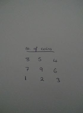
A “grid” with a number of coins on each square
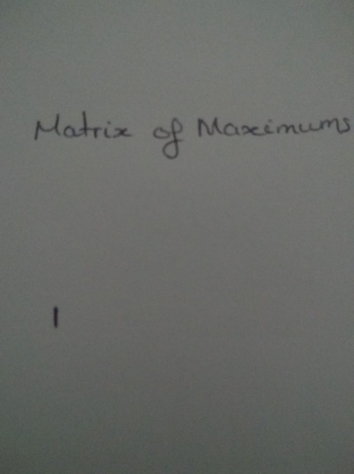
The first entry on our memo
If we start at the bottom left corner and want to travel to the top right in the way prescribed, it’s apparent on inspection that before our first move (while we still stand at 0,0) We would have 1 coin.
Let’s record that on a memo, here that is going to take the form of another matrix which records the maximum possible number of coins for each square.
Now we have our base case, and we know the number of coins on each square- we can proceed by working out the maximums for the bottom row and column (moving in the required way, there is only one path to get to these squares)
For the bottom row, we move sideways- collecting 2 coins and then 3 coins:
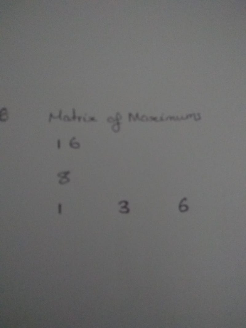
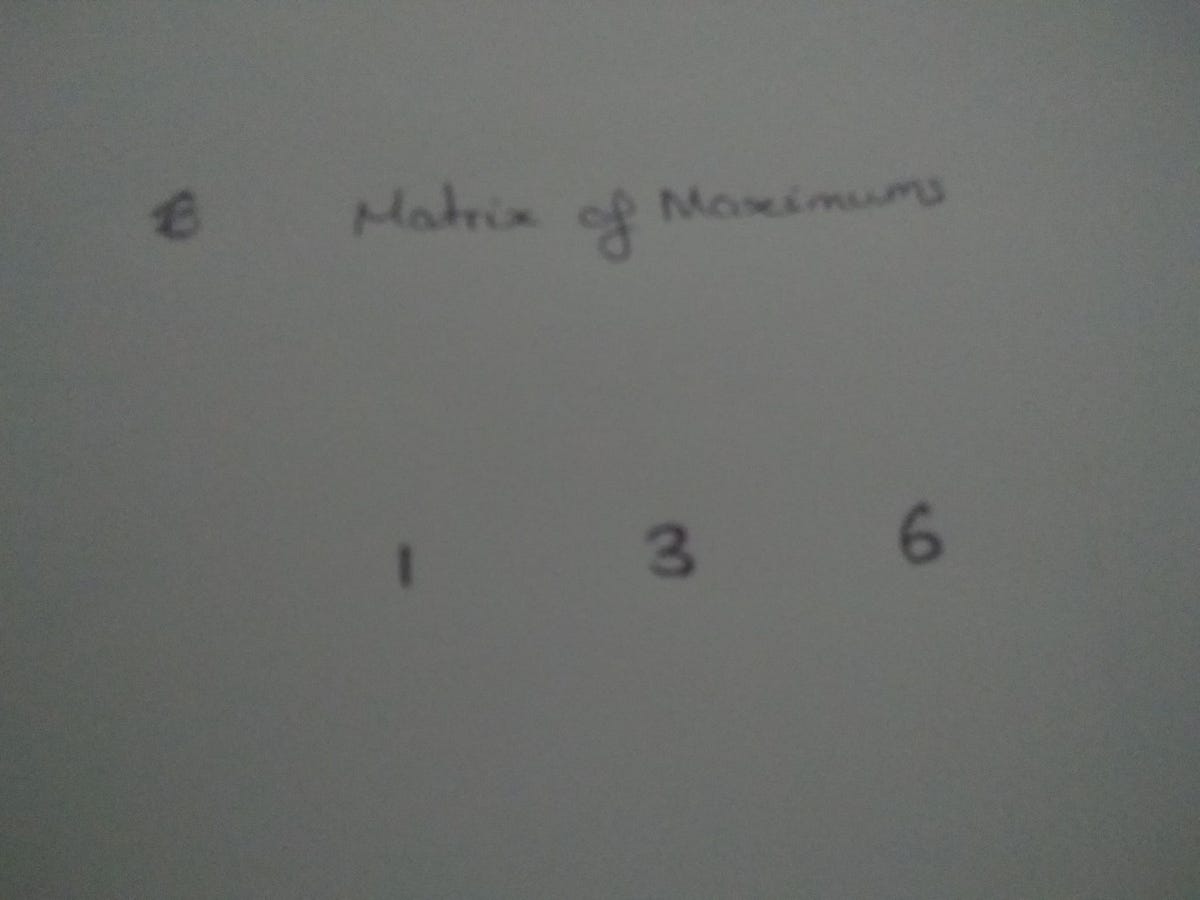

Matrix of maximums: Note that the maximum for a square is the highest maximum for a square prior, plus the number of coins on the square in question
We repeat this process with the first column then we fill in the middle to get the following complete matrix
We can then see that the maximum number of coins is 27. We did this without recursion because we never recomputed our old results.
Now, to do this with code:
function MaxCoins(A){

  //First finding the values of P and Q
  const x_axis = A.length
  const y_axis= A[0].length

  //setting up the "matrix of maximums"

  let memo=[]
  for (let i=0; i<x_axis ; i++){
     memo[i] = []
   }

  //Base Case
  memo[0][0] = A[0][0]

  //Bottom Row

  for (let i=1 ; i<x_axis; i++){
    memo[i][0] = memo[i-1][0]+A[i][0]
  }

  //Bottom Column

  for (let i=1 ; i<y_axis; i++){
    memo[0][i] = memo[0][i-1]+A[0][i]
  }

//Everywhere else
  for (let i=1; i<x_axis; i++){
    for (let k=1; k<y_axis; k++){
       if (memo[i-1][k]>memo[i][k-1]){
          memo[i][k] = memo[i-1][k]+A[i][k]
       }else {
          memo[i][k] = memo[i][k-1]+A[i][k]
       }
    }
  }

  return memo[x_axis - 1][y_axis - 1 ]
 }
This returns 27 as expected.
Conclusion
At the time, working through a problem under time pressure without knowing how to solve it was tough. However, After working out how a solution could be arrived upon, and having had a look at how this method works — overall, this has been a gratifying, and educational experience. I learned something new, that I can take with me into code challenges (and, perhaps, real enterprise code) in the future.


